Portfolio Linear Models for Data Analysis Lab 2: Simple Linear Regression
Lab 2: Simple Linear Regression
Overview of simple linear regression.
library(psych) #describe()
library(PerformanceAnalytics) #chart.correlation()
library(lm.beta) #lm.beta()
library(sjPlot) #tab_model()
library(gridExtra) #grid.arrange()
library(tidyverse)
This lab will be an overview of simple linear regression and was created along side Karen’s lectures and her code.
Simple Linear Regression
The Equation
The equation of simple linear regression is this:
$$Y_i = \alpha + \beta{x}_i + \epsilon_i $$ Expressed as Betas:
$$ Y_i = \beta_0 + \beta{x}_i + \epsilon_i $$
When we are predicting Y, we express the prediction equation as this:
$$\hat Y = a+ b{x} $$
As presented in lecture and lab 1, here is how we would plug in our intercept and slope values into our equations:
# Reading in physics.csv dataset
physics <- read_csv("physics.csv")


#`msat` predicting `physics`
slr_model <- lm(physics~msat,data=physics)
summary(slr_model)
##
## Call:
## lm(formula = physics ~ msat, data = physics)
##
## Residuals:
##     Min      1Q  Median      3Q     Max
## -36.735  -7.484  -0.243   8.980  30.098
##
## Coefficients:
##              Estimate Std. Error t value Pr(>|t|)
## (Intercept) -58.54334   10.46659  -5.593 7.54e-08 ***
## msat          0.27977    0.02112  13.246  < 2e-16 ***
## ---
## Signif. codes:  0 '***' 0.001 '**' 0.01 '*' 0.05 '.' 0.1 ' ' 1
##
## Residual standard error: 12.76 on 193 degrees of freedom
##   (5 observations deleted due to missingness)
## Multiple R-squared:  0.4762,	Adjusted R-squared:  0.4735
## F-statistic: 175.5 on 1 and 193 DF,  p-value: < 2.2e-16
$$ Y = -58.54 + .28{x} $$
An Example
Data from UCLA - Academic Performance Index:
| Variable | Description |
| api00 | Academic Performance Index |
| enroll | School enrollment |
| Meals | Number of free and reduced lunch |
| full | Percentage of teachers will full credentials |
Read in data and view first 6 rows. Here, we are reading in the data directly from the UCLA website:
api <- read.csv(
"https://stats.idre.ucla.edu/wp-content/uploads/2019/02/elemapi2v2.csv") %>%
  select(api00, full, enroll, meals)

#First 6 rows
head(api)
##   api00 full enroll meals
## 1   693   76    247    67
## 2   570   79    463    92
## 3   546   68    395    97
## 4   571   87    418    90
## 5   478   87    520    89
## 6   858  100    343    10
Descriptive Statistics:
describe(api)
##        vars   n   mean     sd median trimmed    mad min  max range  skew
## api00     1 400 647.62 142.25  643.0  645.79 177.17 369  940   571  0.10
## full      2 400  84.55  14.95   88.0   86.60  14.83  37  100    63 -0.97
## enroll    3 400 483.46 226.45  435.0  459.41 202.37 130 1570  1440  1.34
## meals     4 400  60.31  31.91   67.5   62.18  37.81   0  100   100 -0.41
##        kurtosis    se
## api00     -1.13  7.11
## full       0.17  0.75
## enroll     3.02 11.32
## meals     -1.20  1.60
Correlations:
cor(api, method = "pearson", use = "complete.obs") %>%
  round(2)
##        api00  full enroll meals
## api00   1.00  0.57  -0.32 -0.90
## full    0.57  1.00  -0.34 -0.53
## enroll -0.32 -0.34   1.00  0.24
## meals  -0.90 -0.53   0.24  1.00
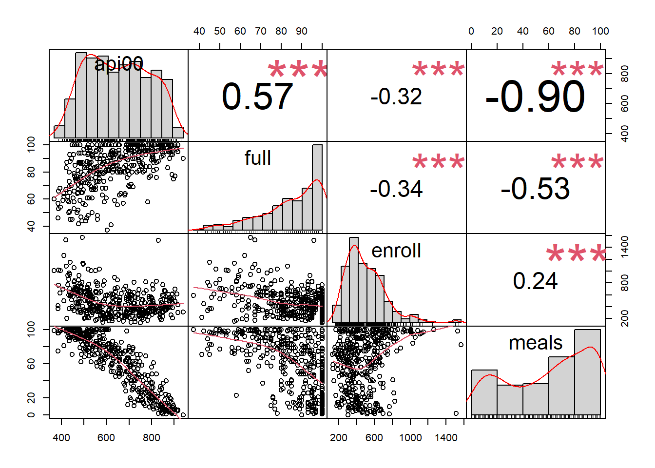
A fancier correlation matrix from Karen’s lecture and code:
chart.Correlation(api, histogram=TRUE, pch=19)
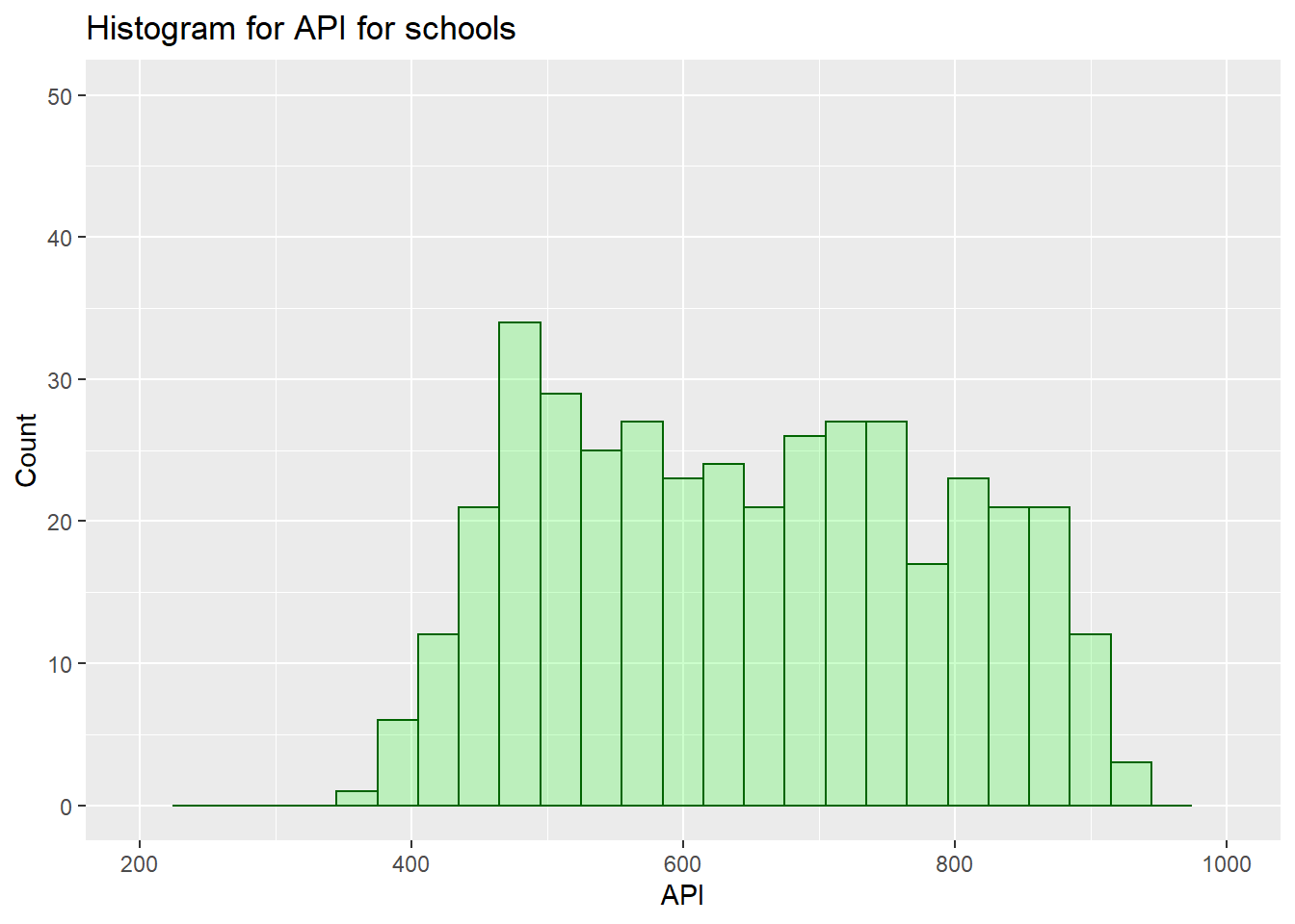
Histogram for API schools:
api %>%
  ggplot(aes(x = api00)) +
  geom_histogram(col="dark green",
                 fill="green",
                 alpha = .2,
                 binwidth = 30) +
  labs(title="Histogram for API for schools", x="API", y="Count") +
  xlim(c(200, 1000)) +
  ylim(c(0,50))
Simple linear regression:
[Research question]{.ul}: Does school enrollment predict school API?
m1 <- lm(api00 ~ enroll, data = api)
summary(m1)
##
## Call:
## lm(formula = api00 ~ enroll, data = api)
##
## Residuals:
##     Min      1Q  Median      3Q     Max
## -285.50 -112.55   -6.70   95.06  389.15
##
## Coefficients:
##              Estimate Std. Error t value Pr(>|t|)
## (Intercept) 744.25141   15.93308  46.711  < 2e-16 ***
## enroll       -0.19987    0.02985  -6.695 7.34e-11 ***
## ---
## Signif. codes:  0 '***' 0.001 '**' 0.01 '*' 0.05 '.' 0.1 ' ' 1
##
## Residual standard error: 135 on 398 degrees of freedom
## Multiple R-squared:  0.1012,	Adjusted R-squared:  0.09898
## F-statistic: 44.83 on 1 and 398 DF,  p-value: 7.339e-11
Standardized Beta Coefficients:
lm.beta(m1)
##
## Call:
## lm(formula = api00 ~ enroll, data = api)
##
## Standardized Coefficients::
## (Intercept)      enroll
##          NA  -0.3181722
Nicely presented regression table using tab_model():
tab_model(m1, show.std = TRUE, show.stat = TRUE, show.zeroinf = TRUE)
| api 00 | ||||||
|---|---|---|---|---|---|---|
| Predictors | Estimates | std. Beta | CI | standardized CI | Statistic | p |
| (Intercept) | 744.25 | 0.00 | 712.93 – 775.57 | -0.09 – 0.09 | 46.71 | <0.001 |
| enroll | -0.20 | -0.32 | -0.26 – -0.14 | -0.41 – -0.22 | -6.70 | <0.001 |
| Observations | 400 | |||||
| R2 / R2 adjusted | 0.101 / 0.099 | |||||
Here, we can see both unstandardized and standardized regression coefficients.
Outliers
Outlier Detection
From Karen’s slides:
There are various ways to diagnose outliers:
[Distance (residuals]{.ul}): is useful in identifying potential outliers in the dependent variable (Y).
[Leverage]{.ul} (h~i~): is useful in identifying potential outliers in the independent variable (x’s). Leverage identifies outliers with respect to the X values
[Influence:]{.ul} combines distance and leverage to identify unusually influential observations (use Cook’s D).
Distance (residuals)
The studentized residual:
$$ e_{s_i} = \frac{e_i}{s \sqrt{1-h_i}} = \frac{e_i}{\sqrt{MS_{Error}(1-h_i)}} $$
The student residual identifies outliers with respect to their y values.
To find studentized residuals in R:
library(MASS) #We use the MASS package for this, I don't like this package because it masks the `select` function from dplyr (tidyverse). After we find studentized residuals, let's detach it.

#Using API data (m1)
stud_res <- as.data.frame(studres(m1)) %>%
  rename("stud_res" = "studres(m1)")

#View first 6 rows
head(stud_res)
##      stud_res
## 1 -0.01397309
## 2 -0.60544501
## 3 -0.88459579
## 4 -0.66480228
## 5 -1.20436717
## 6  1.35389271
#Let's detach the package so we don't get any errors moving forward
detach("package:MASS")
Let’s plot the predictor variable (enroll) and the corresponding studentized residuals:
plot(api$enroll, as.matrix(stud_res), ylab='Studentized Residuals', xlab='Predictor')
abline(0,0)

We can see that there is a studentized residual with an absolute value greater than (or pretty close to) 3 (top right). Let’s combine the studentized outliers with our dataset to get an idea of which observation is the outlier here.
We can add a column by using tidyverse::add_column() and then sort by descending using arrange() and desc() .
new_api <- api %>%
  add_column(stud_res)

#Sort stud_res by descending:
new_api %>%
  arrange(desc(stud_res)) %>%
  head()
##     api00 full enroll meals stud_res
## 8     831   96   1513     2 2.993100
## 242   903  100    696     2 2.222040
## 86    912   97    611     6 2.160181
## 196   894   93    615    13 2.030676
## 339   892   78    602     2 1.995923
## 239   897   75    547    11 1.950388
We can see that observation 8 has a studentized residual of about 3.
Leverage
$$ h_i = \frac{1}{N} + \frac{(x_i - \overline{x})^2}{\sum_{i = 1}^{N}(x_i - \overline{x})^2} $$
To calculate a leverage score for each x in the data set in R, we use the hatvalues() function to calculate the leverage for each observation in the model:
#Using API example (m1)
hats <- as.data.frame(hatvalues(m1)) %>%
  rename("hats" = "hatvalues(m1)")
head(hats)
##          hats
## 1 0.005232891
## 2 0.002520470
## 3 0.002882500
## 4 0.002709463
## 5 0.002565239
## 6 0.003464328
We can also plot the leverage values for each observation:
plot(hatvalues(m1), type = 'h')
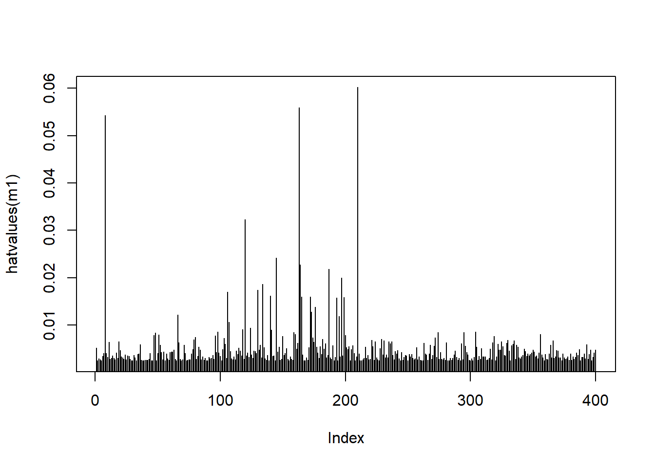
This plot shows some spikes in leverage values.
Let’s find out the cut off.
Leverage (h~i~) values greater than \(\frac{3(p+1)}{N}\) are considered influential ($p$ = number of predictors, \(N\) = sample size)
To calculate the leverage cut-off scores in R:
# Using our API example

#Number of predictors: 1
p <- 1
#Sample Size: 400
n <- 400

leverage <- (3*(p+1))/n
leverage
## [1] 0.015
To find the leverage values above our cut off (Influential values):
influential <- hats %>%
  filter(hats > leverage)
influential
##           hats
## 8   0.05430490
## 106 0.01704568
## 120 0.03227648
## 130 0.01742135
## 134 0.01868945
## 140 0.01620497
## 145 0.02414863
## 163 0.05592762
## 164 0.02274105
## 165 0.01599870
## 172 0.01599870
## 187 0.02180846
## 193 0.01574307
## 197 0.01995080
## 199 0.01589615
## 210 0.06020004
We can see that observation 8 has the highest leverage value.
If we want to remove all leverage values greater than the cut off from our api dataset:
new_api_no_lev <- api %>%
  filter(hats < leverage)
Influence
Combines distance and leverage to identify unusually influential observations (use Cook’s D).
Cook’s distance measure is defined as:
$$ Cook’s D = \frac{(e_{s_i})^2}{p + 1} * \frac{h_i}{1-h_i} $$
Where \(e_{s_i}\) is the studentized residual, \(p\) = number of predictors, and \(h_i\) is the leverage for observation for the \(i\)th observation.
To find Cook’s D in R:
First let’s create a scatterplot for our model (enroll by api00):
api %>%
  ggplot(aes(x = enroll, y = api00)) +
  geom_point() +
  geom_smooth(method = "lm") +
  theme_minimal()
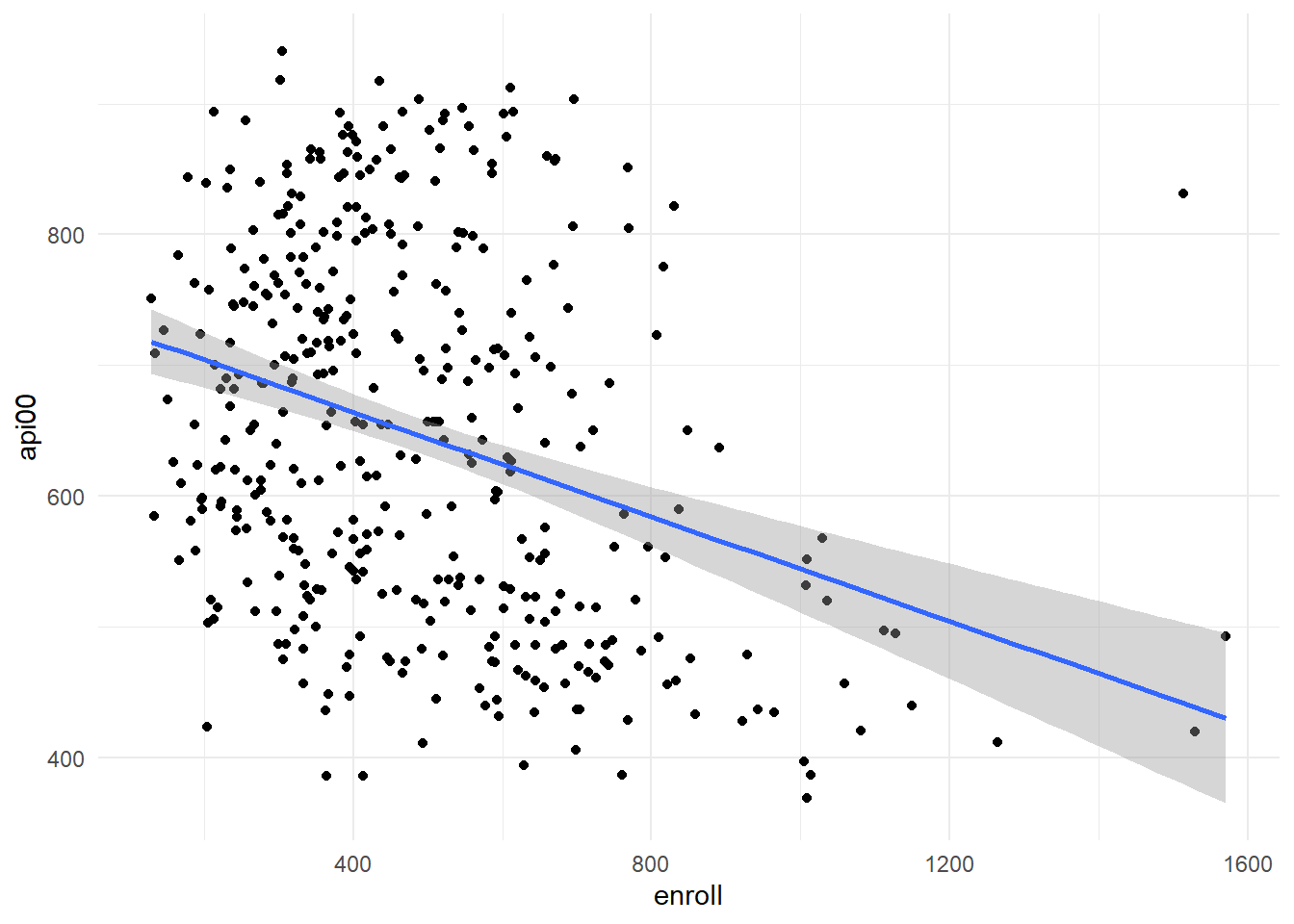
We can clearly see an outlier that is shifting our datapoints to the left. Let’s calculate and plot Cook’s D using R (This is Karen’s code!):
#Cacluating Cook's D
cooksd <- cooks.distance(m1)

#Plotting Values
plot(cooksd, pch="*",
     cex=2,
     main="Influential Obs by Cooks distance") # plot
abline(h = 4*mean(cooksd, na.rm=T),
       col="red")  # add cutoff line
text(x=1:length(cooksd)+1,
     y=cooksd,
     labels=ifelse(cooksd>4*mean(cooksd, na.rm=T),
                   names(cooksd),""),
     col="red")  # add labels
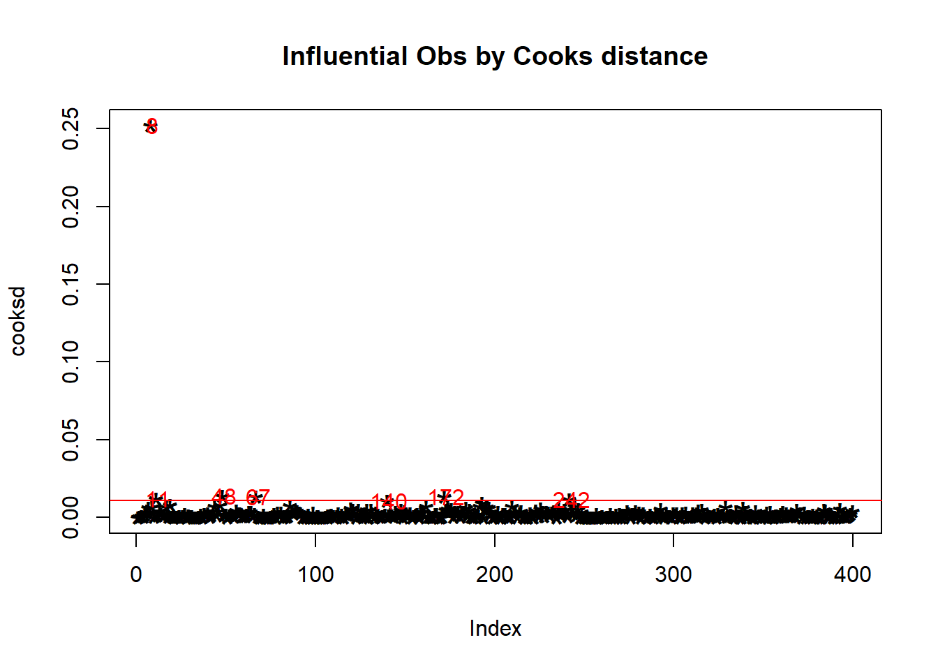
As we’ve noted multiple times, observation 8 has proven to be the outlier in this dataset.
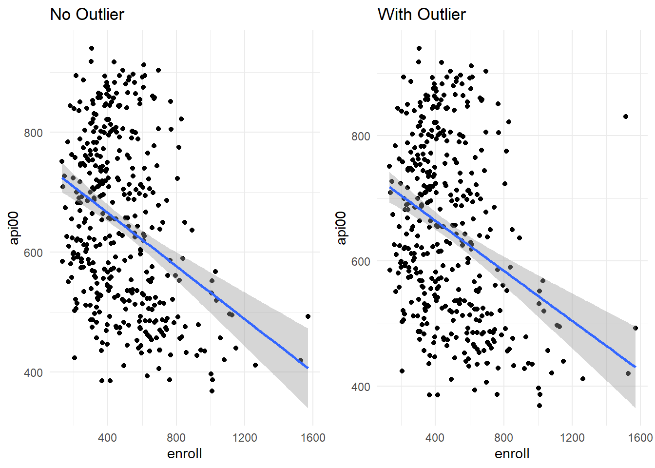
Let’s remove the outlier (row 8) using slice() and compare scatterplots (using the gridExtra:grid.arrange() to look at the plots side by side):
#Remove outlier
api_no_outlier <- api %>%
  slice(-8)

# Scatterplot without the outlier
no_outlier <- api_no_outlier %>%
  ggplot(aes(x = enroll, y = api00)) +
  geom_point() +
  geom_smooth(method = "lm") +
  labs(title = "No Outlier") +
  theme_minimal()

#Scatterplot with outlier
outlier <- api %>%
  ggplot(aes(x = enroll, y = api00)) +
  geom_point() +
  geom_smooth(method = "lm") +
  labs(title = "With Outlier") +
  theme_minimal()

grid.arrange(no_outlier, outlier, ncol = 2)
We can also rerun and compare regression models:
#Rerun regression
m2 <- lm(api00 ~ enroll, data = api_no_outlier)
summary(m2)
##
## Call:
## lm(formula = api00 ~ enroll, data = api_no_outlier)
##
## Residuals:
##      Min       1Q   Median       3Q      Max
## -286.945 -111.413   -5.914   95.955  303.286
##
## Coefficients:
##              Estimate Std. Error t value Pr(>|t|)
## (Intercept) 753.23324   16.05899  46.904  < 2e-16 ***
## enroll       -0.22057    0.03036  -7.266 1.97e-12 ***
## ---
## Signif. codes:  0 '***' 0.001 '**' 0.01 '*' 0.05 '.' 0.1 ' ' 1
##
## Residual standard error: 133.7 on 397 degrees of freedom
## Multiple R-squared:  0.1174,	Adjusted R-squared:  0.1152
## F-statistic:  52.8 on 1 and 397 DF,  p-value: 1.975e-12
tab_model(m2, show.std = TRUE, show.stat = TRUE, show.zeroinf = TRUE)
| api 00 | ||||||
|---|---|---|---|---|---|---|
| Predictors | Estimates | std. Beta | CI | standardized CI | Statistic | p |
| (Intercept) | 753.23 | -0.00 | 721.66 – 784.80 | -0.09 – 0.09 | 46.90 | <0.001 |
| enroll | -0.22 | -0.34 | -0.28 – -0.16 | -0.44 – -0.25 | -7.27 | <0.001 |
| Observations | 399 | |||||
| R2 / R2 adjusted | 0.117 / 0.115 | |||||
#Compare to model with outlier
summary(m1)
##
## Call:
## lm(formula = api00 ~ enroll, data = api)
##
## Residuals:
##     Min      1Q  Median      3Q     Max
## -285.50 -112.55   -6.70   95.06  389.15
##
## Coefficients:
##              Estimate Std. Error t value Pr(>|t|)
## (Intercept) 744.25141   15.93308  46.711  < 2e-16 ***
## enroll       -0.19987    0.02985  -6.695 7.34e-11 ***
## ---
## Signif. codes:  0 '***' 0.001 '**' 0.01 '*' 0.05 '.' 0.1 ' ' 1
##
## Residual standard error: 135 on 398 degrees of freedom
## Multiple R-squared:  0.1012,	Adjusted R-squared:  0.09898
## F-statistic: 44.83 on 1 and 398 DF,  p-value: 7.339e-11
tab_model(m1, show.std = TRUE, show.stat = TRUE, show.zeroinf = TRUE)
| api 00 | ||||||
|---|---|---|---|---|---|---|
| Predictors | Estimates | std. Beta | CI | standardized CI | Statistic | p |
| (Intercept) | 744.25 | 0.00 | 712.93 – 775.57 | -0.09 – 0.09 | 46.71 | <0.001 |
| enroll | -0.20 | -0.32 | -0.26 – -0.14 | -0.41 – -0.22 | -6.70 | <0.001 |
| Observations | 400 | |||||
| R2 / R2 adjusted | 0.101 / 0.099 | |||||
What are the differences in output? Coefficients? R^2^ ?