Text Data Analysis - Michael Scott Version

A text and sentiment analysis on the "Dinner Party" episode of The Office.

code

library(tidyverse)
library(tidytext)
library(textdata)
library(pdftools)
library(ggwordcloud)
library(here)
library(pander)
library(ggthemes)
here::i_am("dinnerparty.txt")

The Office - Season 4 x Episode 9: The Dinner Party

The Dinner Party

Read in the text transcript

Source: https://www.officequotes.net/no4-09.php

dinner_text <- read_delim(here("dinnerparty.txt"), 
                          "\t", escape_double = FALSE, col_names = FALSE, 
                          trim_ws = TRUE) %>% 
  rename(lines = X1)

Each row is a a line of the transcript for each character.

Example: First line from the episode is from Stanley Hudson:

dinner_line1 <- dinner_text[1,]

dinner_line1 %>% 
  pander()

        lines

Stanley: This is ridiculous.

Tidy Data

I separated the character names and their lines into two columns, character and line, separated by colon.
Removed the last four rows that are not character’s lines but stage direction.
I filtered the characters to include the characters that spoke the most words.

dinner_tidy <- dinner_text %>% 
  separate(col = lines, into = c("character", "line"), sep = ":") %>% 
  slice(-(283:288)) %>% 
  filter(character %in% c("Andy", "Angela", "Dwight", "Michael", "Hunter's CD", "Jan", "Jim", "Pam"))

Tokenize

Here, we get word counts for each character for the episode.

dinner_tokens <- dinner_tidy %>% 
  unnest_tokens(word, line)

dinner_wordcount <- dinner_tokens %>% 
  count(character, word)

Remove stop words

Most of the words in the transcript are stop words. To remove them, we use anti_join and the stop_words function.

dinner_nonstop_words <- dinner_tokens %>% 
  anti_join(stop_words)

We then recount with the stopwords removed.

nonstop_counts <- dinner_nonstop_words %>% 
  count(character, word)

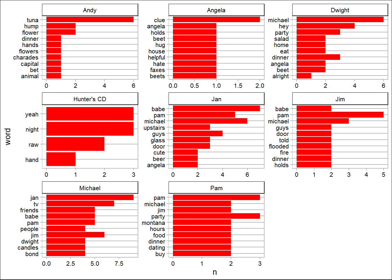
Top 10 Words

Here, we find the top 10 words that each character said during that episode.

top_10_words <- nonstop_counts %>% 
  group_by(character) %>% 
  arrange(-n) %>% 
  slice(1:10)


top_10_words %>% 
  group_by(word) %>% 
  ggplot() +
  geom_bar(aes(reorder(word, n), n), stat = 'identity', fill = "red") +
  facet_wrap(~character, scales = "free") +
  coord_flip() +
  theme_calc() +
  labs(x = 'word')

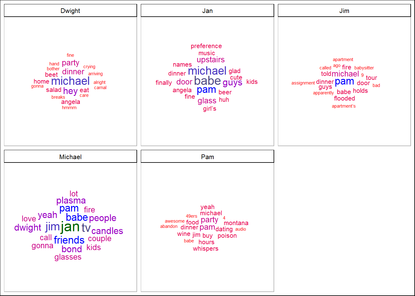
Word Cloud

Let’s make a word cloud for the top 5 characters who spoke the most:

Michael, Jan, Jim, Pam, Dwight

nonstop_counts %>% 
  group_by(character) %>% 
  count() %>% 
  arrange(desc(n)) %>% 
  pander()

character n

Michael 275

 Jan       190 

 Jim       88  

 Pam       72

Dwight 38

Angela 21

Andy       20

Hunter’s CD 4

dinner_top5 <- nonstop_counts %>% 
  filter(character %in% c("Michael", "Jan", "Jim", "Pam", "Dwight")) %>% 
  group_by(character) %>% 
  arrange(-n) %>% 
  slice(1:20)

cloud <- ggplot(data = dinner_top5, aes(label = word)) +
  geom_text_wordcloud(aes(color = n, size = n), shape = "diamond") +
  scale_size_area(max_size = 6) +
  scale_color_gradientn(colors = c("red","blue","darkgreen")) +
  facet_wrap(~character) +
  theme_calc()

cloud

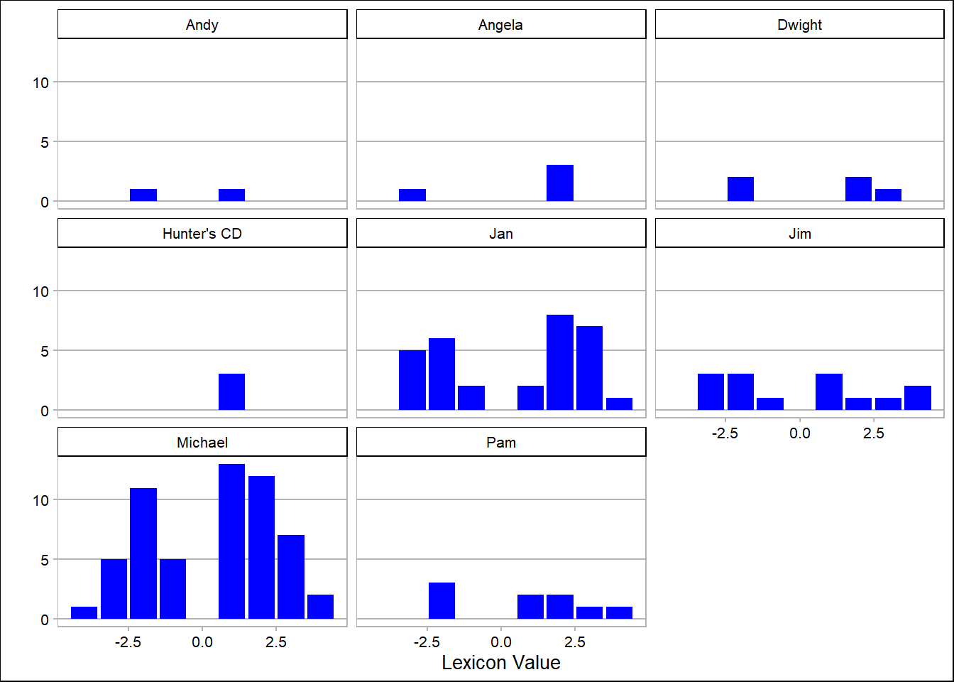
Sentiment Analysis

#afinn lexicon
get_sentiments(lexicon = "afinn")

Sentiment analysis with afinn:

First, bind words in dinner_nonstop_words to afinn lexicon:

dinner_afinn <- dinner_nonstop_words %>% 
  inner_join(get_sentiments("afinn"))

Then, we find counts based on afinn lexicon and plot them:

afinn_counts <- dinner_afinn %>% 
  count(character, value)

# Plot them: 
ggplot(data = afinn_counts, aes(x = value, y = n)) +
  geom_col(fill = "blue") +
  facet_wrap(~character) +
  theme_calc() +
  labs(y = "", x = "Lexicon Value")

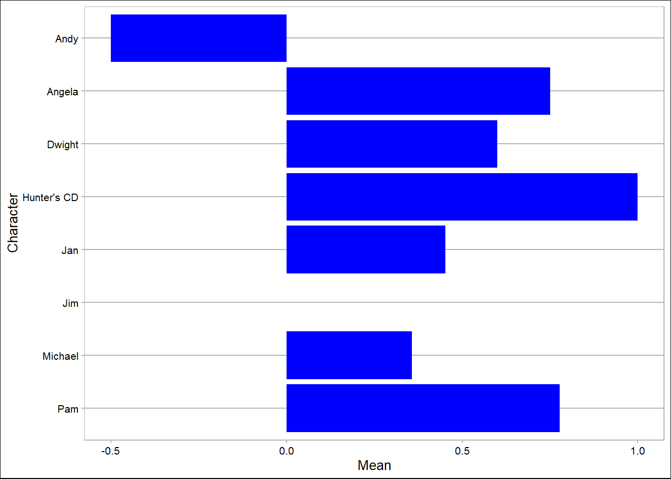
# Find the mean afinn score by characeter: 
afinn_means <- dinner_afinn %>% 
  group_by(character) %>% 
  summarize(mean_afinn = mean(value))

ggplot(data = afinn_means, 
       aes(x = fct_rev(as.factor(character)), 
           y = mean_afinn)) +
  geom_col(fill = "blue") +
  coord_flip() +
  theme_calc() +
  labs(x = "Character", y = "Mean")